In Section 7.9.2 of Real-Time Rendering, we discussed deferred rendering approaches, including “partially-deferred” methods where some subset of shader properties are written to buffers.  Since publication, a particular type of partially-deferred method has gained some popularity.  There are a few different variants of this approach that are worth discussing; more details “under the fold”.

First, I’ll briefly discuss the “classic” or “full” deferred shading approach.  For this discussion, I will assume a shading equation which looks like this:

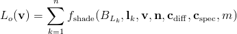
The equation uses the notation from our book.  It means that the output radiance from a surface point in the view direction (in other words, the pixel color) is equal to a sum over n point/directional light sources.  For each light source, the summed quantity is the result of a shading function which depends on (in order of appearance) the light intensity/color at that surface point, the light direction vector, the view vector, the normal vector, the diffuse surface color, the specular surface color, and a specular spread factor such as a Blinn-Phong cosine power.  This equation does not include any ambient or environmental lighting terms – those are handled separately in deferred shading systems.

The two quantities that vary per light are the direction vector l and the intensity/color B_L.  In game engine terms, B_L is equal to the light color times its intensity times the distance attenuation factor at the shaded point (in the book, we use E_L; the two are related thus: B_L=E_L/π).  B_L is an RGB-valued, HDR quantity (as opposed to RGB-valued quantities like c_diff or c_spec whose values are restricted to lie between 0 and 1).

Given this shading equation, deferred shading is typically applied in the following phases:

1. Render opaque scene geometry, writing normal vector, diffuse color, specular color, and specular spread factor into a deep frame buffer or G-Buffer.  Since these will not fit into a single render target, this requires multi-render-target (MRT) support.  Write ambient or environment lighting results into an additional accumulation buffer.
2. Apply the effects of light sources by rendering 2D or 3D shapes covering each light’s area of effect (this relies on lights having a finite area of effect – true for most lights used in real-time applications, although not strictly physically correct).  Non-local light sources such as the Sun are applied in full-screen passes.  When rendering each “light shape”, evaluate the shading equation for that light, reading the G-Buffer channels as textures.  Accumulate the results of the shading equation into the accumulation buffer, using additive blending.  The depth-buffer from phase #1 is typically used to find the world- or view-space position of each shaded point.  This position is used to compute light distance attenuation and to lookup any shadow maps.
3. Render any semitransparent geometry using non-deferred shading.

The results are in principle equivalent to the traditional, non-deferred shading approach (in practice buffer range and precision issues may cause artifacts).  Notably, full deferred shading is used in Killzone 2 as well as the upcoming Starcraft II.

There are several downsides to this approach – the G-Buffer consumes a lot of storage and bandwidth, and the application is restricted to the same shading equation everywhere on the screen.  Handling multi-sample anti-aliasing (MSAA) can also be difficult.  However, deferred shading also has significant advantages; it  solves the light combinatorial problem, and most importantly, it reduces light computation to the absolute minimum (each light is only computed for those pixels that it actually affects).

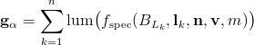
By generalizing the idea of deferred rendering, storage and bandwidth usage can be considerably reduced.  Any sub-expression of a shading equation can be rendered into a buffer and used in a later pass.  One of the most common approaches utilizes the fact that many shading equations have separate diffuse and specular terms, each modulated by a color:

The symbol that looks like an “x” inside a circle is another bit of notation from our book; it denotes a piecewise vector (in this case, RGB) multiplication.

This structure is utilized by a partial deferred shading approach which is most commonly called deferred lighting.  Deferred lighting is applied in the following phases:

1. Render opaque scene geometry, writing normal vector n and specular spread factor m into a buffer.  This “n/m buffer” is similar to a G-Buffer but contains less information.  The values fit into a single output color buffer, so MRT support is not needed.
2. Render “light shapes”, evaluating diffuse and specular shading equations and writing the results into separate specular and diffuse accumulation buffers.  This can be done in a single pass (using MRT), or in two separate passes.  Environment and ambient lighting can be accumulated in this phase with a full-screen pass.
3. Render opaque scene geometry a second time, reading the diffuse and specular accumulation buffers from textures, modulating them with the diffuse and specular colors and writing the end result into the final color buffer.  If not accumulated in the previous phase, environment and ambient lighting are applied in this phase.
4. Render any semitransparent geometry using non-deferred shading.

This is equivalent to refactoring the shading equation thus:

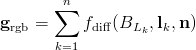
Or, looking separately at the accumulation phase:

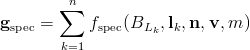
and the reconstruction phase:

This technique was first described in a GDC 2004 presentation by Rich Geldreich, Matt Pritchard, and John Brooks.  It was used in Naughty Dog‘s Uncharted: Drake’s Fortune, and Insomniac‘s Resistance 2.  Insomniac detailed their development in an internal presentation, and described the final system in a recent GDC talk.  Crytek also adopted this approach in CryEngine 3.  Compared to a full deferred shading approach, this has some advantages.  It can be used on older hardware that does not support MRT, the processing for each light is cheaper, and bandwidth and storage requirements are much reduced.  Some variation in shading equations is also possible, by replacing c_diff or c_spec with various expressions.

A variant on this technique renders a full G-Buffer in phase #1, and then applies the specular and diffuse colors to the accumulation buffers in a full-screen pass in phase #3 instead of rendering the opaque geometry a second time.  I believe S.T.A.L.K.E.R.: Clear Sky uses this variant.

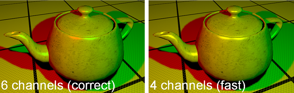
Storage and bandwidth requirements can be further reduced by compacting the separate diffuse and specular RGB accumulation buffers into a single RGBA buffer (reducing the number of distinct color channels used from 6 to 4).  The CryEngine 3 presentation also discusses this approach.  They accumulate the full RGB diffuse term, but only the luminance of the specular term (into the alpha channel).  The specular chromaticity information is discarded, and the chromaticity of the diffuse term is used to approximate that of the specular term.  This is plausible, but not 100% correct – imagine a red light source and a green light source shining onto a surface from different directions.  The diffuse term will be yellow, but the specular term should have two separate highlights – one red and one green.  With this approximation, both highlights will be yellow.

This can be seen in one of the images from the CryEngine 3 presentation, used here with Crytek‘s kind permission:

In an appendix at the end of this post, I give some details on a possible implementation of 4-channel deferred lighting.

Deferred lighting (especially the 4-channel variant) is somewhat like the light pre-pass approach developed by Wolfgang Engel (described on his blog and in two chapters of the recently released ShaderX⁷ book).  The idea of a light pre-pass has helped inspire much of the recent work on deferred lighting, and the two techniques are broadly similar.  However, the details show some significant differences.  The basic “G-Buffer” given in ShaderX7 contains only the surface normal n.  Since the specular spread m is not available during the accumulation phase, some other specular spread value (either fixed or derived from the light source) is used, and the value of m is applied in the reconstruction phase.  Since there is no way to do this correctly (specular terms have nonlinear dependence on m), a number of variant shading models are given to approximate the desired result.  These are ad hoc and each has drawbacks; for example, at least one (equation 8.5.6) has lights affecting each other’s attenuated intensity contribution, instead of each light having its own independent, additive effect.

Appendix A – Four-Channel Deferred Lighting Implementation

The Crytek presentation does not explain exactly how the specular is reconstructed.  The most correct method would probably be to transform the accumulated diffuse lighting into a space like CIELUV, apply the diffuse chromaticity to the accumulated specular luminance, and transform the result into RGB.  That would be quite expensive; a cheaper method would be to divide the accumulated RGB diffuse term by its luminance and multiply by the accumulated specular luminance.  Again looking separately at the accumulation phase:

and the reconstruction phase:

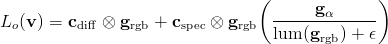
The epsilon in the denominator is a very small value put there to avoid divides by zero.  The function lum() converts an RGB value into its luminance; it computes a simple weighted average of the R, G and B channels.  If the RGB quantity is in linear space, and the RGB primaries are those used in standard monitors and televisions, then the equation is:

This method of reconstructing specular should produce the correct result with one light, and will preserve the correct specular luminance with multiple lights.

Appendix B – Deferred Lighting with Example Shading Model

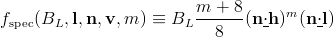
It is interesting to see how this discussion applies to a specific shading model.  I will use a physically based model from Chapter 7 of our book:

The half-vector h is a vector halfway between the light vector l and the view vector v; to compute it, just add the two and normalize the result.  The underlined dot notation is not from RTR3, it’s something I just made up to concisely express the commonly-used “clamped dot product”, which is a dot product with negative values clamped to 0.  R_F is the Fresnel reflectance function; it modifies the material’s characteristic specular color c_spec towards white as the dot product of l and h goes from 1 to 0.

Unfortunately, this shading equation is not in the right form for deferred lighting, due to the Fresnel function modifying the specular color for each light.  A solution to this is to use a different dot product in the Fresnel function; the dot product of v and n instead of that of l and h.  This is not strictly correct, but it is a reasonable approximation (the two dot products are equal in the middle of the specular highlight) and it makes the specular color invariant over light sources, which lets us refactor this equation into the form needed for deferred lighting:

(here I’ve used the Schlick approximation to R_F to compute a modified specular color)

Although a Fresnel term results in more realistic shading than a constant specular color, it does have one downside for deferred lighting.  It requires accessing the n/m buffer in phase #3, slightly increasing bandwidth usage and restricting opportunities for reusing the buffer.  If this is a concern, the Fresnel function can be replaced with a constant specular color.

The (m+8)/8 term in f_spec can take large values for materials with high specular powers, possibly preventing the use of a low-precision buffer for specular accumulation.  One solution is to move that term from f_spec to c_spec – applying it in phase #3 instead of phase #2.  If you are using a Fresnel function, the value of m is readily available after reading the n/m buffer (see above).